Objective
To develop a computational method that allows:
Segmenting existing roads in an input image. That is, given an aerial image, provide a binary mask with road pixels set to 1 and the rest to 0.
For a set of test images, provide a set of quantitative evaluation metrics for the segmentation appropriate for the target application, using the corresponding ground truth.
Workflow
Load the input images and each ground truth.
Experiment with possible operations on the original images that allow us to obtain relevant point features.
- Different filters and image processing techniques were tested to find those best adapted to road segmentation.
Creation of a feature vector for each pixel of the aerial image.
- The values obtained with the operations from the previous step will characterize each pixel of the image.
Division into training and test sets.
- 80% of the images are divided for training and the remaining 20% for model evaluation.
Creation and training of a classifier with the obtained feature vectors and labels.
- The classifier architecture is defined, different models are tested.
Classifier evaluation with the test image set, and road segmentation is obtained.
Evaluation metrics for the classifier are obtained with the test set.
Labels for each pixel of the input image are predicted, and road segmentation is obtained.
The obtained segmentation is visualized and compared with the corresponding ground truth.
The best predictions are subjected to post-processing.
1. Loading the image and ground truth
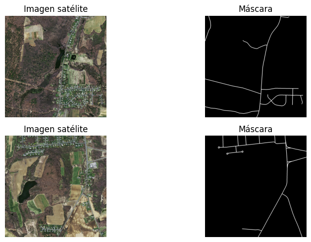
Input aerial image and its ground truth
2. Experimentation for feature extraction
We experimented with different filters and image processing techniques to obtain relevant features that help us segment roads.
3. Feature vector
After experimenting with different filters and image processing techniques, it was decided that the feature vector would consist of the following elements:
R, G, and B channels of the original image to obtain color information.
H and S channels of the image in HSV color space to obtain color information.
Manual thresholding on the b channel (previously expanded)
Otsu thresholding on the H and S channels
Gradient direction and magnitude of the grayscale image.
def features(image):
    """
    Calculates features of a satellite image for road detection.

    Args:
        image (ndarray): Input image.

    Returns:
        array: Image features.
        - R, G, and B channels of the original image to obtain color information.
        - Manual thresholding on the b channel (previously expanded)
        - Otsu thresholding on the H and S channels
        - Gradient direction and magnitude of the original image with a sigma of 1 and discretization to 36 directions.
    """

    ## Convert image to grayscale
    image_gray = skimage.color.rgb2gray(image)

    ## Calculate gradient and orientation with a sigma of 1 and discretization to 36 directions
    grad = gradient_magnitude(image_gray, sigma=1)
    orient = gradient_orientation(image_gray, sigma=1, discrete_angles=8)

    ## Convert image to HSV
    image_hsv = skimage.color.rgb2hsv(image)

    ## Get H and S channels
    channel_h = image_hsv[:, :, 0]
    channel_s = image_hsv[:, :, 1]

    ## Threshold H and S channels using Otsu
    threshold_h = skimage.filters.threshold_otsu(channel_h)
    threshold_s = skimage.filters.threshold_otsu(channel_s)

    ## Convert image to LAB
    image_lab = skimage.color.rgb2lab(image)
    # Get the b channel
    channel_b = image_lab[:, :, 2]
    # Normalize b channel to [0, 1] range
    channel_b = (channel_b + 128) / (127 + 128)
    # Expand b channel histogram
    channel_b = exposure.rescale_intensity(channel_b, in_range='image', out_range=(0, 1))
    # Threshold the b channel using a manual threshold
    threshold_b = 0.4

    ## Create a list of features
    features = [image[:, :, i] for i in range(3)] + \
                      [channel_h] + \
                      [channel_s] + \
                      [channel_b < threshold_b] + \
                      [channel_h > threshold_h] + \
                      [channel_s > threshold_s] + \
                      [grad, orient]

    ## Reshape features to have the same shape
    features = np.array(features)
    features = np.transpose(features, (1, 2, 0))

    return features
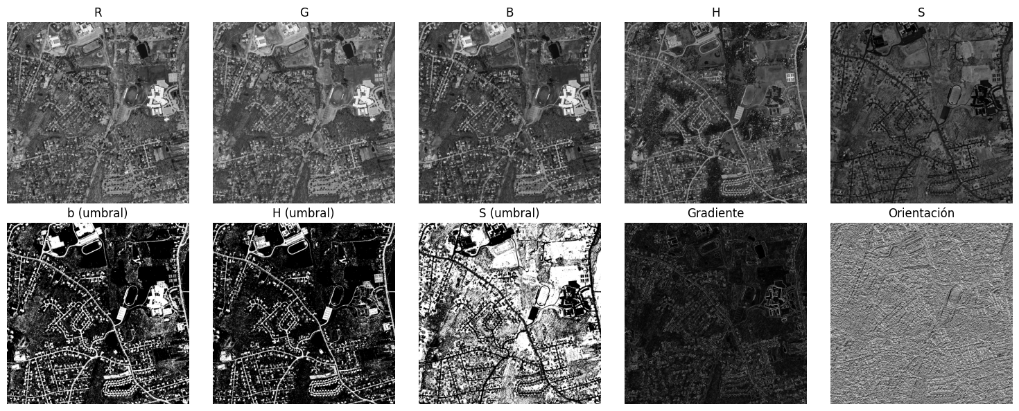
Example of the feature vector constructed by the classifier
4. Creation of training and test sets
We divide the satellite images into a training set (80%) and a test set (20%). We have dispensed with functions for splitting training and test sets, as the size of the images is small but disparate, and a random split is not necessary.
Actually, if the goal is only to segment roads in the specific images, dividing the data would not be necessary, it would be sufficient to train a model with all images regardless of whether it overfits; in fact, overfitting might even be useful.
In this work, we decided to divide the data to try to train a model that can generalize to other road images, not just the specific images offered to us.
5. Classifier creation
The following function will serve to create our binary classifier (road / not road) using a convolutional neural network.
def model1(input_shape):
    inputs = layers.Input(shape=input_shape)

    x = layers.Conv2D(32, (3, 3), activation='relu', padding='same')(inputs)

    x = layers.Conv2D(16, (3, 3), activation='relu', padding='same')(x)

    x = layers.Conv2D(1, (1, 1), activation='sigmoid', padding='same')(x)

    outputs = layers.Reshape((input_shape[0], input_shape[1]))(x)
    model = models.Model(inputs=inputs, outputs=outputs)

    model.compile(optimizer=optimizers.Adam(learning_rate=0.001),
              loss=losses.BinaryCrossentropy(),
              metrics=[
                  metrics.BinaryAccuracy(name='accuracy'),
                  metrics.Precision(name='precision'),
                  metrics.Recall(name='recall'),
                  metrics.AUC(name='auc')])

    return model
Clarification:
Our fundamental metric for evaluating performance will be AUC (Area Under Curve). Our problem is a clear example of a binary classification problem where classes are highly imbalanced; the vast majority of pixels are not roads.
For this reason, accuracy is not an appropriate metric as it can be misleading. For example, if the classifier predicts that all pixels are background, accuracy will still be high (it will have correctly predicted the majority of pixels) but it won’t have learned anything.
However, the AUC metric indicates the ratio between false positives and true positives, making it a more appropriate metric for our problem. It will be 1 if the classification is perfect and 0.5 if it’s random.
Note: It should be noted that using this metric does not avoid the imbalance problem, it just helps us evaluate the classifier’s performance.
In case of wanting to mitigate the imbalance problem, techniques such as oversampling, assigning weights to give more importance to the minority class (road), or defining specific loss functions for this problem could be applied.
In this case, although we tried modifying the loss function in some of the created models (present in the final part of the Notebook), we reached satisfactory training without this technique. Regardless, we must be aware of the existing problem.
We create the classifier and train it with the training set. This model receives the 1500x1500x10 matrix directly as input, no image flattening is performed. Each image constitutes a batch.
## Create the model
INPUT_SHAPE = (1500, 1500, 10)
model = model1(input_shape=INPUT_SHAPE)

## Model summary
model.summary()

## Train the model
history = model.fit(x_train, y_train, epochs=5, batch_size=1)

## Save the model
model.save("modelo1.keras")
Conclusion
We created a convolutional network with two layers of 32 and 16 neurons respectively, with relu activation, and another layer with 1 neuron and sigmoid activation. A more complex architecture was tested, but increasing complexity did not offer significant improvements and considerably increased computational cost, making training practically impossible. We used
binary_crossentropyloss and Adam optimizer. Training was conducted for 5 epochs. The metric used to evaluate classifier performance is AUC (Area Under Curve).The network’s output is a value between 0 and 1 indicating the probability that the pixel is a road; later this is processed to obtain binary segmentation.
6. Classifier evaluation on the test image set
We load the model.keras classifier and evaluate it with the test set. We obtain the evaluation metrics.
Conclusion:
We obtained an AUC of 0.89, which indicates the classifier performs well. We will qualitatively evaluate the segmentation obtained on the test images.
We define a function to visualize the results. The satellite image, ground truth, and the segmentation obtained by the classifier will be shown. Note that the output of our model, and therefore the prediction, is a probability between 0 and 1 for each pixel, so a threshold will be applied to convert the output to a binary image.
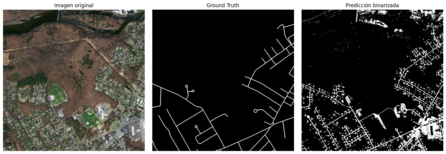
Segmentation comparison on test image (1)
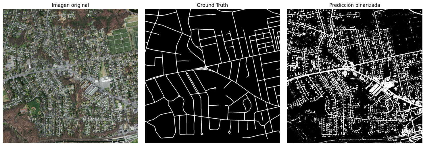
Segmentation comparison on test image (2)
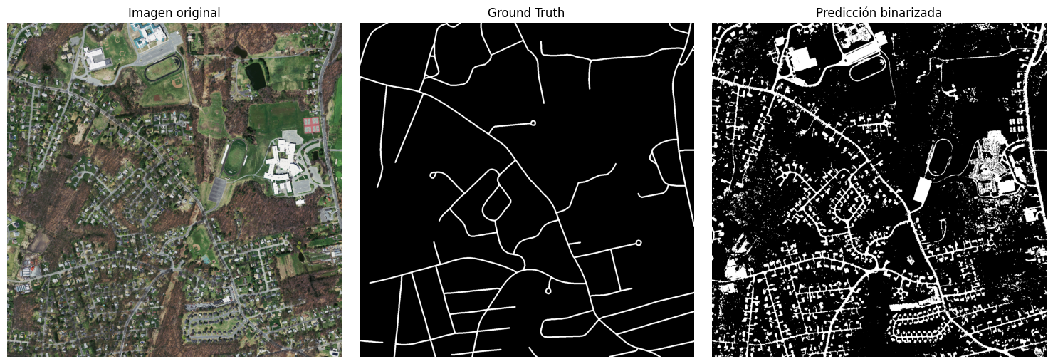
Segmentation comparison on test image (3)
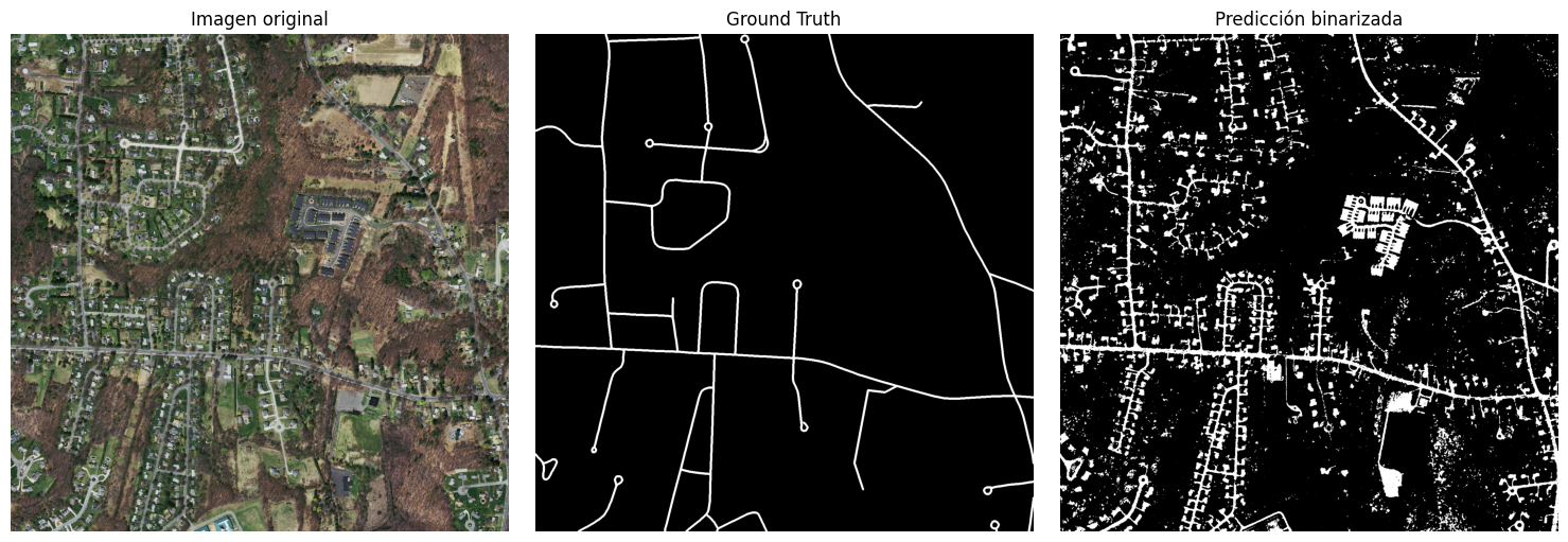
Segmentation comparison on test image (4)
7. Post-processing of the obtained segmentation
We will try to improve the obtained segmentation through post-processing. To do this, we will test a series of techniques and choose those that offer a good result.
Finally, our post-processing consists of:
- Threshold of 0.6 for binarizing the image obtained by the classifier.
- Removal of connected components smaller than 50 pixels.
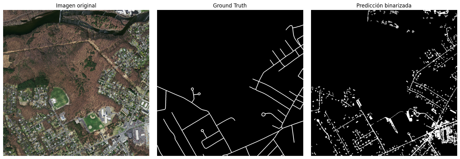
Final segmentation after post-processing (1)
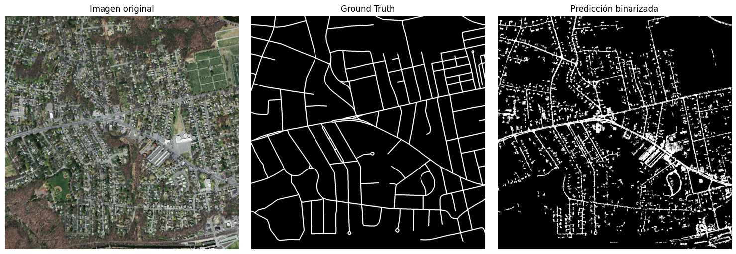
Final segmentation after post-processing (2)
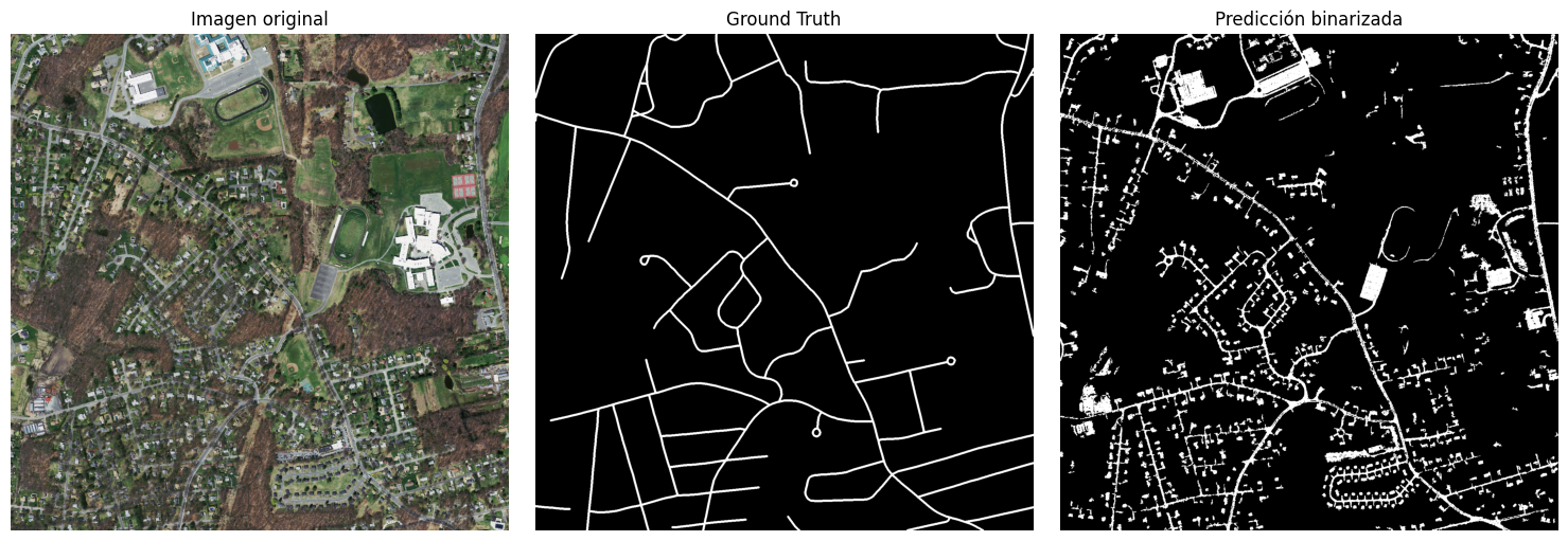
Final segmentation after post-processing (3)
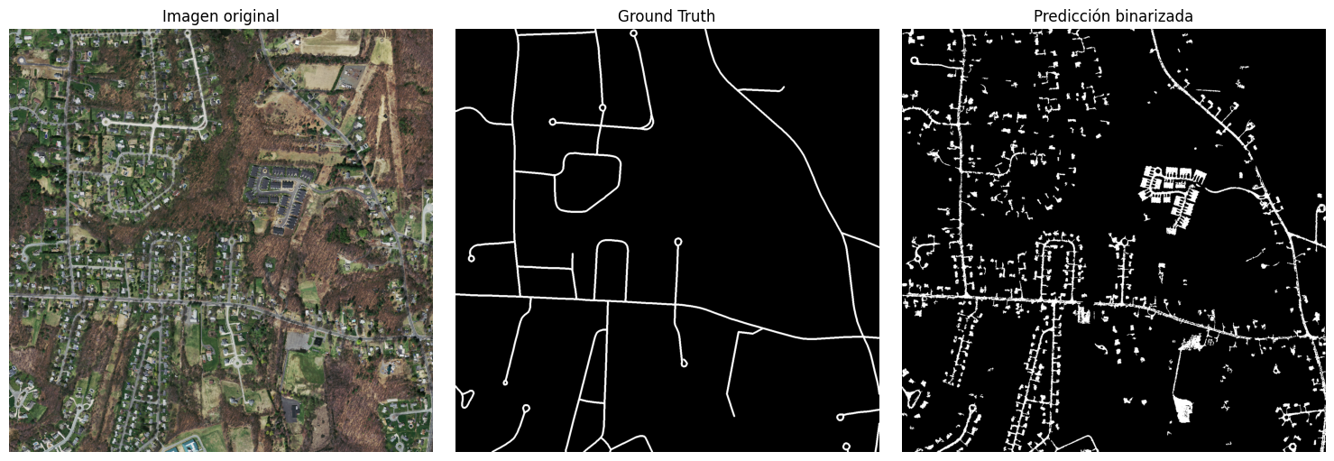
Final segmentation after post-processing (4)
Final Conclusions
General assessment:
Quantitatively, the segmentation obtained by the classifier is quite good, with an AUC result of 0.89.
The segmentation obtained by the classifier is not perfect but quite good. Segmentation errors are observed in the obtained binary image. These errors are mainly noise pixels that have been classified as road and small discontinuities, but there are also larger structures that it detects as roads.
Model weaknesses. Errors:
Our model identifies a large number of roofs as roads; we did not create a model capable of effectively differentiating between the two. The same happens with industrial warehouses or large commercial surfaces.
There are discontinuities in the predicted roads that cannot be eliminated in post-processing.
Our binary image has minimal noise points that cannot be eliminated with connected component labeling.
There are several roads that are not detected, which are roads in the ground truth and, more importantly, can be identified as such in the satellite image.
Model strengths:
Our segmentations effectively differentiate roads from forest trails or firebreaks.
Roadways not determined by the ground truth are obtained, but they are effectively roads to the naked eye in the satellite image.
All narrow roads between houses or, conversely, extensive paved areas (such as parking lots) are identified as roads by our model.
Our model generalizes well; the segmentation is good on the images it has learned but does not overfit to them and is able to predict those in the test set.
More Information
For more details on the project, the notebook with the complete code and the results obtained in each step of the process can be consulted in the project’s GitHub repository